![]()
Table Of Contents
Previous topic
PyMP Tutorial 1. MP decomposition with Unions of MDCT
Next topic
PyMP Tutorial 3. Greedy decomposition variants
![]()
PyMP Tutorial 1. MP decomposition with Unions of MDCT
PyMP Tutorial 3. Greedy decomposition variants
We now assume you’re familiar with PyMP and the different Pursuit types that can be performed In this tutorial we illustrate the advantages of RSSMP in an audio compression context.
A much more detailed discussion on this can be found in the paper , let’s just introduce the basics
To encode an approximation  of
of  atoms, one needs to encode two things:
- The indexes of the atoms in the dictionary
- Their weights
The simplest encoding scheme is to encode each atom separately. In this setup the cost of encoding
an atom’s index is fixed and directly linked to the size of the dictionary. The cost of encoding
an atom’s weight is also fixed if we use a static midtread quantizer with  steps.
There are many more efficient way of encoding sparse representation. One way is to adapt the quantization of the weights to the exponentially decreasing bound of MP as done by Frossard et al 2004.
Another way is to use en entropic coder or any other source coding method after the quantization step. Finally, atom indexes can be redundant over time (especially when considering signal frames closely related in time) All these scheme are situation-dependant and beyond the scope of this tutorial.
Indexes coding costs are linked to the dictionary size, but in the case of adaptative pursuits (such as LOMP) an additionnal parameter (e.g. a local optimal time-shift) must be transmitted as side-information.
Let us perform a MP decomposition of a 1 second audio exceprt of Glockenspiel using a 3xMDCT dictionary:
>>> from PyMP.mdct import Dico, LODico
>>> from PyMP.mdct.rand import SequenceDico
>>> from PyMP import mp, mp_coder, Signal
>>> sig = Signal('data/ClocheB.wav', mono=True)  # Load Signal
>>> sig.crop(0, 4.0 * sig.fs)     # Keep only 4 seconds
>>> # atom of scales 8, 64 and 512 ms
>>> scales = [(s * sig.fs / 1000) for s in (8, 64, 512)]
>>> sig.pad(scales[-1])
>>> # Dictionary for Standard MP
>>> mp_dico = Dico(scales)
>>> # Launching decomposition, stops either at 20 dB of SRR or 2000 iterations
>>> mp_approx, mp_decay = mp.mp(sig, mp_dico, 20, 2000, pad=False)
This should be relatively fast, the algorithm stops when it reaches 20 dB of SRR and a number of atoms determined by:
>>> mp_approx.atom_number
565
From the mp_approx object constructed we can now evaluate a (theoretical) rate and an associated distorsion by quantizing
the atoms weights and counting the cost of both indices and weights. To do that, we use the simple_mdct_encoding() method
in the mp_coder module. Here’s an example where we set a target of 8kbps with a midtread uniform quantizer with  steps
steps
>>> snr, bitrate, quantized_approx = mp_coder.simple_mdct_encoding(mp_approx, 8000, Q=14)
And we can check the results:
>>> print "%f, %f" % (snr, bitrate)
20.011907, 3472.723833
In other words, we achieved a 20 dB SNR with a (theoretical) 3.4 kbps bitrate. We can change the coder properties,
in particular the number of quantizing steps (recall this is and not directly Q!!):
>>> snr, bitrate, quantized_approx = mp_coder.simple_mdct_encoding(mp_approx, 8000, Q=5)
>>> print "%f, %f" % (snr, bitrate)
12.556648, 997.297883
Indeed we have reduced the bitrate, but increased the distorsion. We can also fix the bitrate at a lower value:
>>> snr, bitrate, quantized_approx = mp_coder.simple_mdct_encoding(mp_approx, 2000, Q=14)
>>> print "%f, %f" % (snr, bitrate)
16.036869, 2003.730919
The coder stopped when the given bitrate was reached, yieled a higher distorsion. If you wonder how many atoms where used:
>>> quantized_approx.atom_number
326
In order to listen to the results, you’ll need to save the approximant as wav files:
>>> quantized_approx.recomposed_signal.write('data/ClocheB_quantized_2kbps.wav')
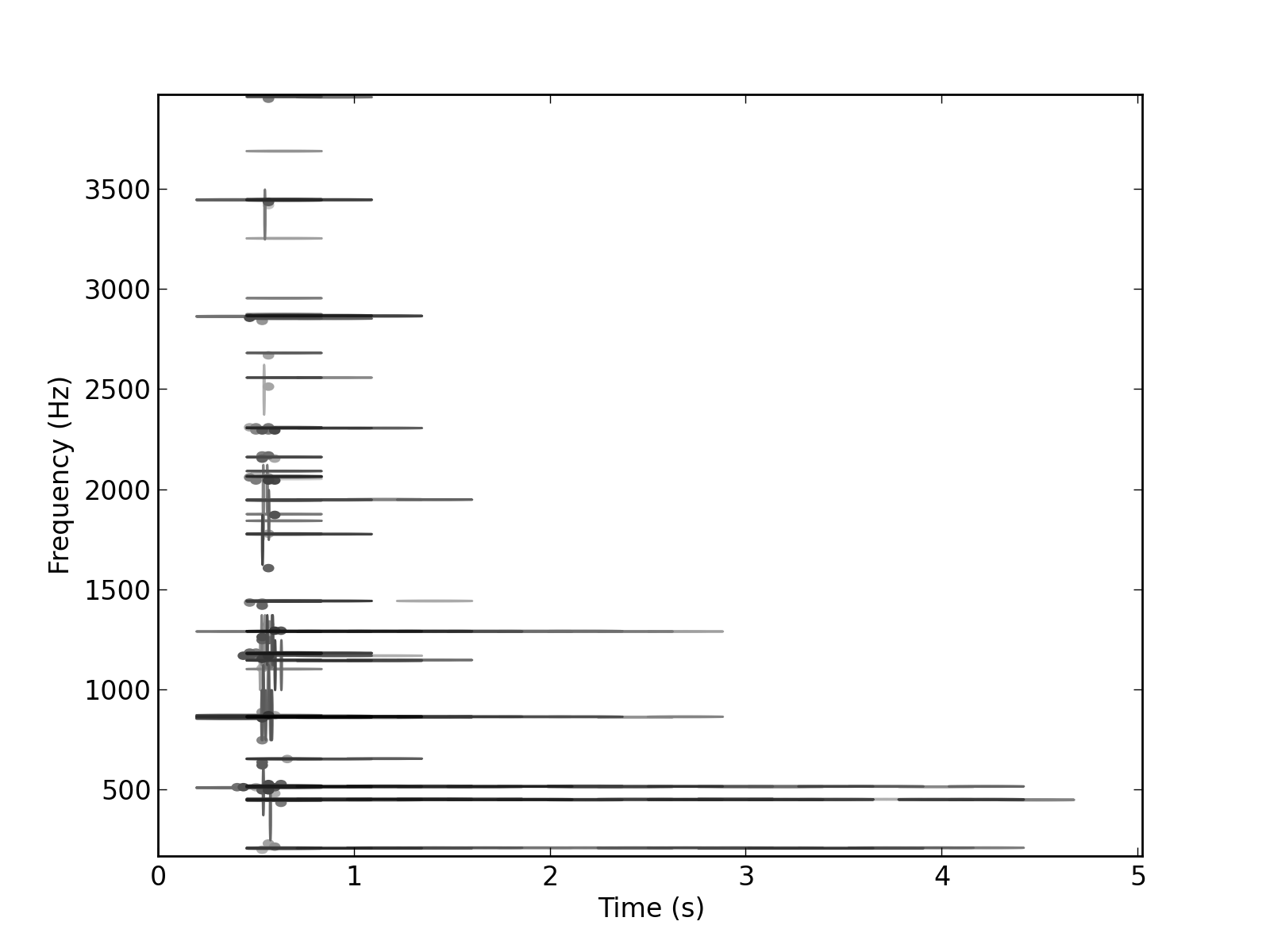
But a simple Time-Frequency plot already tells you there’s going to be some highly disturbing artefacts:
(Source code, png, hires.png, pdf)
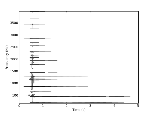
Energy has appeared BEFORE the impact on the bell, this phenomemnon is called pre-echo artefact and is very common when using this type of dictionaries. Only two way to get rid of it:
- Increase the number of atoms (but since we want to compress that’s not a good idea here)
- Select Atoms that have a better fine correlation to the signal. This is the topic of the next example.
Running a locally-optimized MP in an equivalent configuration accounts to using the appropriate dictionary.
>>> lomp_dico = LODico(scales)
>>> lomp_approx , lompDecay = mp.mp(sig, lomp_dico, 20, 2000, pad=False)
Warning
beware to set the option pad to False. Otherwise zeroes are added by default to the signal edges each time you call MP on the same Signal object, this can mess up the bitrate since it is in bps!
An estimation of the SNR and bitrate achieved is done using the same function simple_mdct_encoding() but with the shift_penalty argument set to True in order to take the additionnal parameter cost into account
>>> lomp_snr, lomp_bitrate, lomp_quantized_approx = mp_coder.simple_mdct_encoding(lomp_approx, 2000, Q=14, shift_penalty=True)
Then one can check that the encoding is more efficient:
>>> print "%f, %f" % (lomp_snr, lomp_bitrate)
18.310387, 2006.372657
For the same bitrate of 2 kbps, we now have an SNR of nearly 20 dB where a standard MP yielded a mere 16 dB. Each atom is more expensive, but also creates less dark energy. One can verify that the coder has used a lower number of Locally-optimized atoms:
>>> (quantized_approx.atom_number , lomp_quantized_approx.atom_number)
(326, 249)
Using RSS MP, one need not encode the additionnal time-shift parameter per atom, since we assume the pseudo-random sequence of subdictionaries is known both at the coder and decoder side. This is possible because this sequence is not signal-dependant.
>>> from PyMP.mdct.rand import SequenceDico
>>> rssmp_dico = SequenceDico(scales, 'random', seed=42)
>>> rssmp_approx = mp.mp(sig, rssmp_dico, 20, 2000, pad=False) [0]
>>> rssmp_snr, rssmp_bitrate, rssmp_quantized_approx = mp_coder.simple_mdct_encoding(rssmp_approx, 2000, Q=14)
Now we can check that RSSMP atoms are much more efficient at representing the signal than the ones selected in a fixed dictionary, but the cost of each atom is the same thus:
>>> print "%f, %f" % (rssmp_snr,rssmp_bitrate)
18.931437, 2003.730919
Note
In order to allow to reproduce results, you can set the seed optionnal parameter of the SequenceDico object
And we can verify:
>>> (quantized_approx.atom_number,  lomp_quantized_approx.atom_number , rssmp_quantized_approx.atom_number)
(326, 249, 326)
You can now compare these approach for different signals and dictionaries either directly with the given SNR and bitrate values, or by listening to the diverse solutions:
>>> lomp_quantized_approx.recomposed_signal.write('data/ClocheB_LOMP_quantized_2kbps.wav')
>>> rssmp_quantized_approx.recomposed_signal.write('data/ClocheB_RSSMP_quantized_2kbps.wav')
And that concludes this tutorial.
here’s the documentation of the method used in this tutorial
Module mp_coder
A collection of method handling the (theoretical) encoding of sparse approximations.
- PyMP.mp_coder.simple_mdct_encoding(app, target_bitrate, Q=7, encode_weights=True, encode_indexes=True, subsampling=1, shift_penalty=False, output_file_path=None, output_all_indexes=False)
Simple encoder of a sparse approximation
Arguments:
- app: a Approx object containing atoms from the decomposition
- target_bitrate: a float indicating the target bitrate. Atoms are considered in decreasing amplitude order.
The encoding will stop either when the target Bitrate it reached or when all atoms of approx have been considered
- Q: The number of midtread quantizer steps. Default is 7, increase this number for higher bitrates
- shift_penalty: a boolean indicating whether LOMP algorithm has been used, and addition time-shift parameters must be encoded
Returns:
- snr: The achieved Signal to Noise Ratio
- bitrate: The achieved bitrate, not necessarily equal to the given target
- quantized_approx: a Approx object containing the quantized atoms