PyMP Tutorial 3. Greedy decomposition variants

There are many variants of the MP algorithm. Only a few of them are directly implemented in PyMP. In the first tutorial, we saw some variants of the selection step (e.g. RSSMP). Here we’re interested in the update step. In order to use this variants, we use the mp.greedy() function of the mp module.

Here’s a example of use with a simple multiscale MDCT dictionary and the standard MP algorithm:

>>> from PyMP.mdct import Dico
>>> from PyMP import mp, Signal
>>> sig = Signal('data/ClocheB.wav', mono=True)  # Load Signal
>>> sig.crop(0, 4.0 * sig.fs)     # Keep only 4 seconds
>>> # atom of scales 8, 64 and 512 ms
>>> scales = [(s * sig.fs / 1000) for s in (8, 64, 512)]
>>> sig.pad(scales[-1])
>>> mp_dico = Dico(scales)
>>> # Launching decomposition, stops either at 20 dB of SRR or 2000 iterations
>>> mp_approx, mp_decay = mp.greedy(sig, mp_dico, 20, 2000, pad=False, update='mp')

This is equivalent to using the mp.mp() method. However, the additionnal update keyword argument allows to change the nature of the update step.

Orthogonal Matching Pursuit

The principle of OMP is to ensure that at each iteration, chosen atom weights are the best possible ones (in a least squares sense). An orthogobnal projection of the residual onto the subspace spanned by all previously selected atoms is thus performed. Original paper is [1]. The keyword to use OMP is omp.

Warning

OMP is extremely resource consuming. You should not try to use it on signals with lengths greater than a few thousand samples. Try the local version instead or GP.

Gradient Pursuit

Gradient Pursuits have been introduced by Blumensath and Davis in [2]. The idea is to replace the costly orthogonal projection by a much more affordable directionnal update step.

Warning

Orthogonal and directionnal pursuits implementation are not compatible (yet) with FullDico is implemented.

Local versions of OMP/GP

Mailhé et al [3] have presented variants of OMP and GP that are much more efficient since they only perform the update in a neighborhood of the last selected atom. For the kind of dictionaries that are implemented in PyMP (i.e. time-localized MDCT and Wavelets), this is a great news. The keyword arguments to use the local OMP is locomp and local GP is locgp

Cyclic Matching Pursuit

Coming Soon!

example

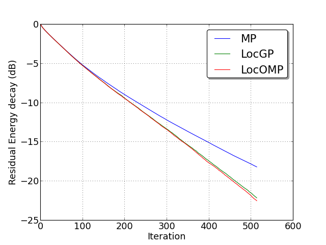
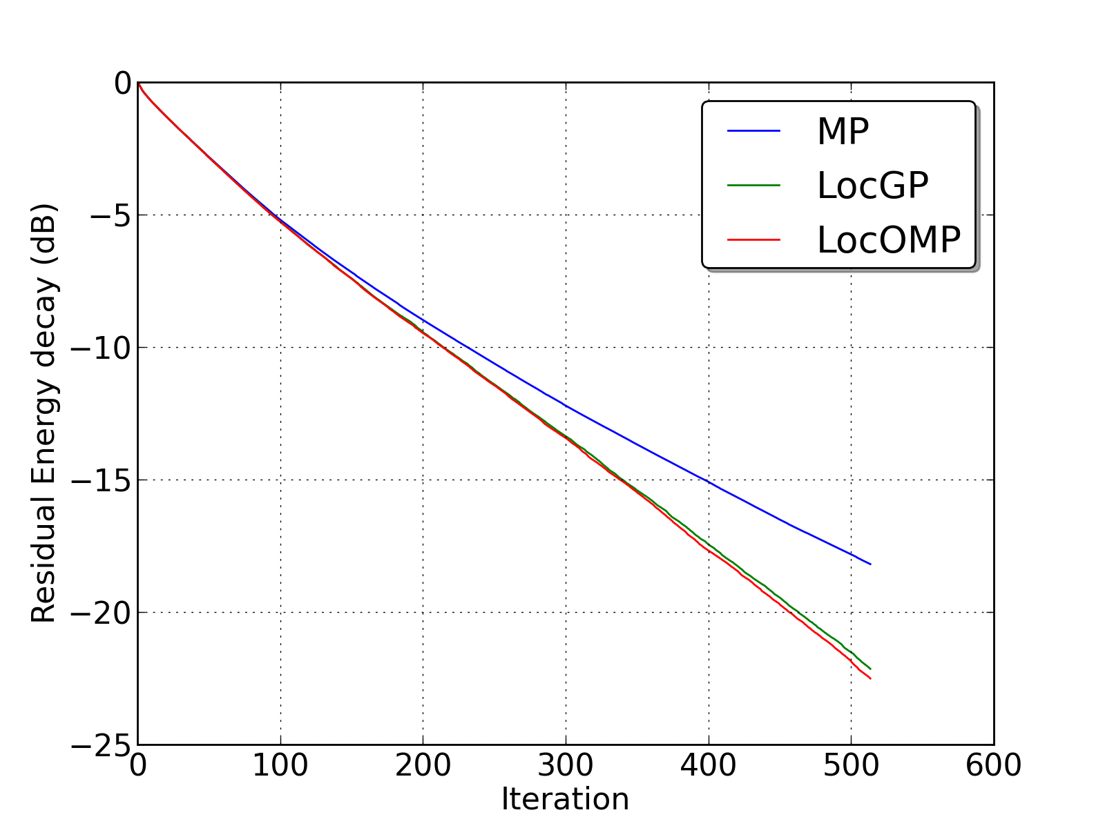
The following example build a k-sparse signal and compares decompositions using MP, locOMP and locGP:

>>> from PyMP import mp, Signal
>>> from PyMP.mdct import Dico
>>> scales = [16, 64, 256]
>>> dico = Dico(scales)
>>> M = len(scales)
>>> L = 256 * 4
>>> k = 0.5*L
>>> # create a k-sparse signal
>>> sp_vec = np.zeros(M*L,)
>>> from PyMP.tools import mdct
>>> random_indexes = np.arange(M*L)
>>> np.random.shuffle(random_indexes)
>>> random_weights = np.random.randn(M*L)
>>> sp_vec[random_indexes[0:k]] = random_weights[0:k]
>>> # initialize true sparse rep
>>> sparse_data = np.zeros(L,)
>>> for m in range(M):
>>>     sparse_data += mdct.imdct(sp_vec[m*L:(m+1)*L], scales[m])
>>> sig = Signal(sparse_data, Fs=8000, mono=True, normalize=True)
>>> sig.data += 0.01 * np.random.random(L,)
>>> sig.pad(scale[-1])
>>> n_atoms = k + 1
>>> # Run the decompositions
>>> app_1, dec1 = mp.greedy(sig, dico, 100, n_atoms, debug=0, pad=False, update='mp')
>>> app_2, dec2 = mp.greedy(sig, dico, 100, n_atoms, debug=0, pad=False, update='locgp')
>>> app_3, dec3 = mp.greedy(sig, dico, 100, n_atoms, debug=0, pad=False, update='locomp')

Plotting the decay with :

>>> plt.figure()
>>> plt.plot(10.0 * np.log10(dec1 / dec1[0]))
>>> plt.plot(10.0 * np.log10(dec2 / dec2[0]))
>>> plt.plot(10.0 * np.log10(dec3 / dec3[0]))
>>> plt.grid()
>>> plt.ylabel('Residual Energy decay (dB)')
>>> plt.xlabel('Iteration')
>>> plt.legend(('MP', 'LocGP', 'LocOMP'))

we have:

(Source code, png, hires.png, pdf)

Bibliography

1 : Pati, Y. C. C., Rezaiifar, R., & Krishnaprasad, P. S. S. Orthogonal Matching Pursuit: Recursive Function Approximation with Applications to Wavelet Decomposition (pdfomp).

Proceedings of the 27 th Annual Asilomar Conference on Signals, Systems, and Computers (pp. 40–44).

2 : Blumensath, T., & Davies, M. . (2008). Gradient Pursuits.

IEEE Transactions on Signal Processing, 56(6), 2370–2382 (pdfgp).

3 : Mailhé, B., Gribonval, R., Vandergheynst, P., & Bimbot, F. (2011). Fast orthogonal sparse approximation algorithms over local dictionaries.

Signal Processing vol 91(12) (2822-2835) (pdfloc).